Here are some of the projects I’ve been involved in the field of Control, Robotics and Machine Learning.
Robotics & Control Projects
- PhD Related
- Work Related
- Master’s Thesis
- Master’s Projects
- Master’s Homeworks
- Cooperative attitude synchronization in satellite swarms: a consensus approach
- A New Method for the Nonlinear Transformation of Means and Covariances in Filters and Estimators
- DC-motor and 4-tanks system control with \(H_\infty\) and \(\mu\)-synthesis techniques
- Implementation of CNN, LSTM and free design of a neural network architecture
Vision-Based Robotic Bronchoscope Localization and Cancer Detection
Simulated example of input camera images and the corresponding output of the realtime robot localization
work in progress…
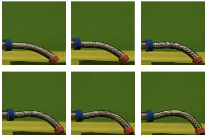
Contact Force Model for Soft Robots
Soft Robots find the best application to robotic surgery, where the compliance of the structure is a key feature to ensure the safety of the patient. However, the compliance of the robot makes the control more challenging, especially when the robot is in contact with the environment and it doesn’t have force sensors.
Here I developed a contact force model for a soft continuum robot, which is able to predict the contact force and the deformation of the robot when in contact with an obstacle.
Short Summary
Goal: Develop a contact force model for a soft robot in contact with the environment
- First, start with modelling the actuators to get the robot dependent mapping, which gives the robot kinematics from the pressure input, together with solving a shape optimization problem to find the best geometric parameters (e.g. shape of the deformed tube)
$$ T( q (p) ) = \small
\begin{bmatrix}
-\sin{q (p)} & \cos{q (p)} & 0 & L^o \dfrac{(1 - \cos{q (p)})}{q (p)}\\[2.5mm]
\cos{q (p)} & \sin{q (p)} & 0 & L^o \dfrac{\sin{q (p)}}{q (p)}\\[2.5mm]
0 & 0 & 1 & 0\\[2.5mm]
0 & 0 & 0 & 1\\[2.5mm]
\end{bmatrix}
\normalsize $$
- Then, use the PCC model to get the robot independent mapping which gives the robot dynamics and the static equilibrium
$$ G(q) + Kq = u_{\tau}(p) + J^T (q) \gamma_e $$
- Finally, combine the static equilibrium with the axial force and tune the final coefficients to get the contact force model
$$ F_{c} = F_{\kappa} + \dfrac{\alpha F_{\epsilon} p}{q} + \beta $$
Last Update: August, 2024
Panda for Hyperthermia
While working at Medlogix I had the possibility of writing the code for controlling the Panda robot from Franka Emika. Here I experimented with many different control techniques such as FBL, impedance and admittance control, to find the best solution for curing cancer with hyperthermia!
One day I asked chatGPT to write the parametric Cartesian equations of an heart and I made the robot follow the trajectory, basically I am just a bridge between two robots.
Here is the Panda spreading some love
Short Summary
Goal: Control the Panda robot for delivering hyperthermia treatment ensuring safety and compliance with the patient body
- Dynamic model of a robot in contact
$$ M(q)\ddot{q} + C(q, \dot{q})\dot{q} + G(q) = u + J^T_r (q)F_r $$
- Impedance control law for constant reference \(r_d\)
By choosing the desired (apparent) inertia equal to the natural Cartesian inertia of the robot we don’t need force feedback, and we can impose the desired damping \(D_m\) and stiffness \(K_m\) to the robot!
$$ u = J^T_r (q)[K_m (r_d - r) -D_m \dot{r}] + G(q) $$
Last Update: January, 2023
MPC for Soft Robots
While I was writing my Master’s thesis I decided to share the code I was using as a new MATLAB Toolbox. SoRoPCC allows you to simulate and control a customizable soft manipulator, both for Shape Control and for Task-space Control, either by controlling the curvature of each CC segment or the position and orientation of the tip of the robot. Moreover it is also embedded with the MPC Toolbox, so you can control the robot using the Model Predictive Control.
Here are some examples of trajectory tracking and set-point regulation of a 3-DOF tentacle.

Top-left is fully actuated; top-right is underactuated on the last CC segment; bottom-left shows how it is possible to control also the orientation; bottom-right is an attempt of sliding on an obstacle to exploit the compliance structure of the robot.
Short Summary
Goal: Executing tasks with a Soft Continuum Robot
- Dynamic model of a soft robot with \(n\) constant curvature segments \(q \in \mathbb{R}^n\)
$$ M(q)\ddot{q} + C(q, \dot{q})\dot{q} + G(q) + D(q)\dot{q} + Kq = A\tau $$
- Discrete time state space representation
$$ x_{k+1} = f(x_k , u_k ) $$ $$ y_k = h(x_k) $$
- MPC control law is obtained by minimizing the cost function (with tail cost) and ensuring the state and input constraints
$$ J_{M}^{N}(x,u) = \sum_{i = 0}^{M-1}l(x(k),u(k)) + \sum_{i = M}^{N-1}l_{\tau}(x(k)) $$
-
What about the closed loop stability?
It has been proved that a sufficiently large prediction horizon guarantees the stability of the system. I was very curious of finding the numerical value of the lower bound \(\bar{N}\).
I learned that if a known stabilizing control law is used to compute the tail cost, this one is a relaxed control Lyapunov function which implies the asymptotic stability and many estimates of the lower bound have been proposed. I used the one proposed by J. Köhler and as stabilizing control laws I used some of those proposed by my friend and colleague P. Pustina -
Playing with the cost index to use the soft robot compliance
The general form that I used for the stage cost is the quadratic norm with respect to a positive definite matrix, both for the state and the input, which is a common choice for the MPC.$$ l(x,u) = ||x(k)||^2_Q + ||u(k)||^2_Q $$
However, I wanted to try to reduce the rigidy of the robot, which is a common issue when applying standard control techniques to soft robots. So I tried to replace the constant weight multiplying the control effort with a row vector \(s = [s_1 , s_2, \cdot \cdot \cdot , s_m]^{T}\) of the same dimension of the control vector, where \(s_i\) is the \(i\)-th input weight, yelding to the cost function
$$\begin{array}{c} J_{ts}(x,u) = \sum_{k = 0}^{M-1} a_1 \norm{h(x(k)) - y_d (k)}^{2} + a_2 \norm{\dot{q}(k)}^{2} + a_3 \norm{s \cdot u(k)}^{2} + \\ a_4 \norm{u(k+1)-u(k)}^{2} + \sum_{k = M}^{N-1} a_5\norm{h(x(k)) - y_d (k)}^{2} + a_6 \norm{\dot{q}(k)}^{2} \end{array}$$
Note that the latters by regulating \(s\) one can “decide” the severity of the underactuation of the system according to the magnitude of the weight. The idea was to dynamically adjust the weights to make the robot more compliant when needed, for example when it is in contact with an obstacle, exploiting the compliance of the structure (see simulation above)
Last Update: March, 2024
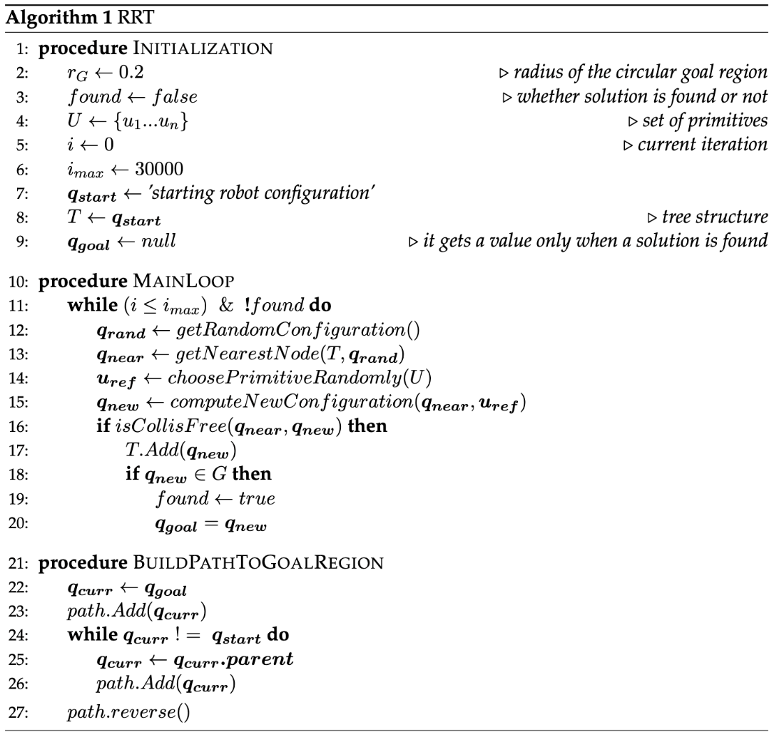
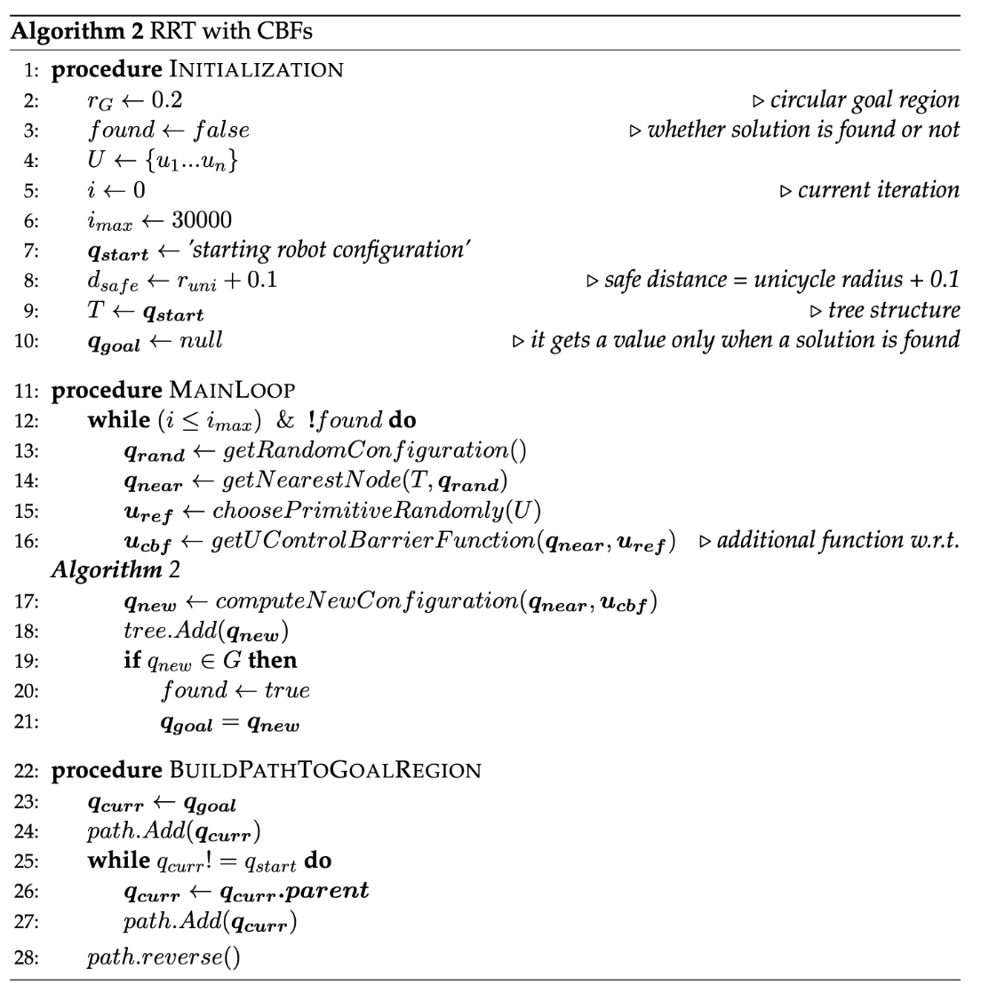
Motion Planning with RRT + CBF
Here is a project about Probabilistic Motion Planning of Unicyle Mobile Robot using Rapidly-exploring Random Tree (RRT) with Control Barrier Functions (CBF)
Here are some examples of the application of the algorithm in four scenes with increasing difficulty
Short Summary
Goal: Plan safe trajectories for a mobile robot using Rapidly-exploring Random Trees (RRT) combined with Control Barrier Functions (CBF). Basically, instead of computing the collision checking as in the standard RRT, we compute the control inputs by using the CBF to modify the provided primitives.
- Kinematic model of the unicyle mobile robot
$$ \begin{bmatrix} \dot{x} \\ \dot{y} \\ \dot{\theta} \end{bmatrix} = \begin{bmatrix} \cos{\theta} \\ \sin{\theta} \\ 0 \end{bmatrix}v + \begin{bmatrix} 0 \\ 0\\ 1 \end{bmatrix}\omega$$
- Choice of the CBF
$$ \mathcal{C}_s := \{x \in \mathbb{R}^2 : \sqrt{(x-x_{obs})^2 + (y - y_{obs})^2} \geq \tau \} $$
- RRT vs RRT + CBF algorithm comparison
Last Update: June, 2021
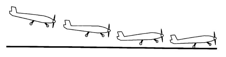
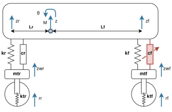
Aircraft Landing Control
Short Summary
GOAL: Design a control system for the landing gear of an aircraft to ensure a safe and autonomous landing.
- The aircraft is modeled as a 7-DOF system with state variable \(x = [ z, z_{wf}, z_{wr}, \theta, x, \omega_{f}, \omega_{r} ]\). The controlled elements are the elevators, the flaps and the active suspension of the front landing gear, together with the breaks of the rear and front gear, yelding to the control input \(u = [ L, u_{\theta}, F_{aereo}, C_r, C_f ]\).
$$ \ddot{z} = -\dfrac{1}{M}\left[ k_f(z_f-z_{wf})+c_f(\dot{z}_{f}-\dot{z}_{wf})+k_r(z_r-z_{wr} )+c_r (\dot{z}_{r}-\dot{z}_{wr}) + L \right ]-g $$
$$ \ddot{z}_{wf} = \dfrac{1}{m_t}\left[ k_f(z_f-z_{wf})+c_f(\dot{z}_{f}-\dot{z}_{wf})-k_t(z_{wf}-y_f ) \right ]-g $$
$$ \ddot{z}_{wr} = \dfrac{1}{m_t}\left[ k_r(z_r-z_{wr})+c_r(\dot{z}_{r}-\dot{z}_{wr})-k_t(z_{wr}-y_r ) \right ]-g $$
$$ \ddot{\theta} = \dfrac{1}{J}\left[ -(k_f l_f) (z_f-z_{wf}) -(c_f l_f) (\dot{z}_{f} - \dot{z}_{wf})+ (k_r l_r) (z_r-z_{wr}) + (c_r l_r) (\dot{z}_{r} - \dot{z}_{wr}) +u_{\theta} \right] $$
$$ \ddot{x} = \dfrac{1}{M}(F_{long_{r}} + F_{long_{f}} - F_{aereo}) $$
$$ \dot{\omega}_{r} = \dfrac{1}{I_{wr}}(C_r - F_{long_{r}R_{t}} - C_{roll_{r}}) $$
$$ \dot{\omega}_{f} = \dfrac{1}{I_{wf}}(C_f - F_{long_{f}R_{t}} - C_{roll_{f}}) $$
- The control system is designed to dived the problem in two pahses: the approach and the touchdown.
The first one, aims to regulate the height \(z_d\) and the angle \(\theta_d\) by means of the lift force \(L\) and it is controlled by a PID controller joint with a Feedback Linearization.
The second one aim to regulate the horizontal velocity \(\dot{x}\) and the angle \(\theta_d\) by using the breaks \(C_r, C_f\) and the active suspension \(u_{\theta}\), this phase is controlled with a Suspension Variational Feedback Controller.
Last Update: July, 2021
Trajectory Tracking of a KUKA LBR 7R
Short Summary
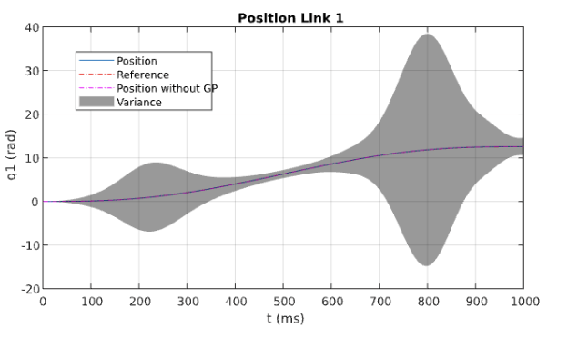
GOAL: When performing a Feedback Linearization (FL) there are always mismatches between the model and the real system, the goal of this porject is to use the Gaussian Process Regression (GPR) to learn the mismatch and to improve the tracking performance of the robot.
- Robot dynamic model
$$ M(q)\ddot{q} + C(q, \dot{q})\dot{q} + G(q) = u $$
- The control law is obtained by using the FL plus a learned correction factor \(\delta u\) from the GPR
$$ u = M(q)(\ddot{q} + K_p (q_d - q) + K_d (\dot{q}_d - \dot{q}) ) + C(q, \dot{q})\dot{q} + G(q) + \delta u $$
- Training the GPR with the data collected from the robot
$$ x_i = [q_i , \dot{q}_i , \ddot{q}_i ]$$
$$ y_i = \delta u_i $$
With the training data we can compute the mean and the variance of the prediction.
Here we used the radial basis function kernel
$$ k(x,x') = \sigma^2 \exp(-\dfrac{1}{2}\norm{x-x'}^2_W) $$
and the Logarithmic Marginal Likelihood with sparsification as the loss function
$$ log\ p(\mathbf{y}|X,\boldsymbol{\theta}) =
(n-m)log(\sigma_n)
+ \sum_{i=1}^m log(l_{M,ii})
+ \frac{1}{2\sigma^2}(\mathbf{y}^T\mathbf{y} - \boldsymbol{\beta}_I^T\boldsymbol{\beta}_I)
+ \frac{n}{2} log (2\pi)
+ \frac{1}{2\sigma^2} trace(K - V^T V) $$
Last Update: July, 2020
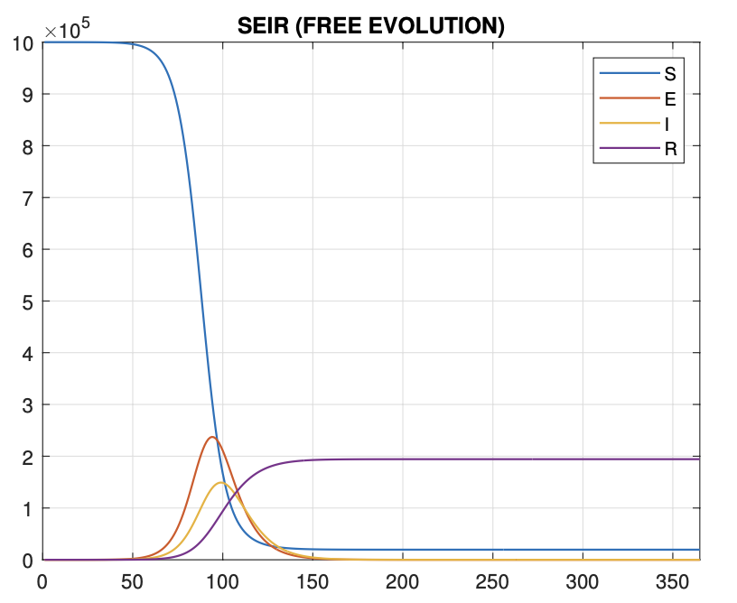
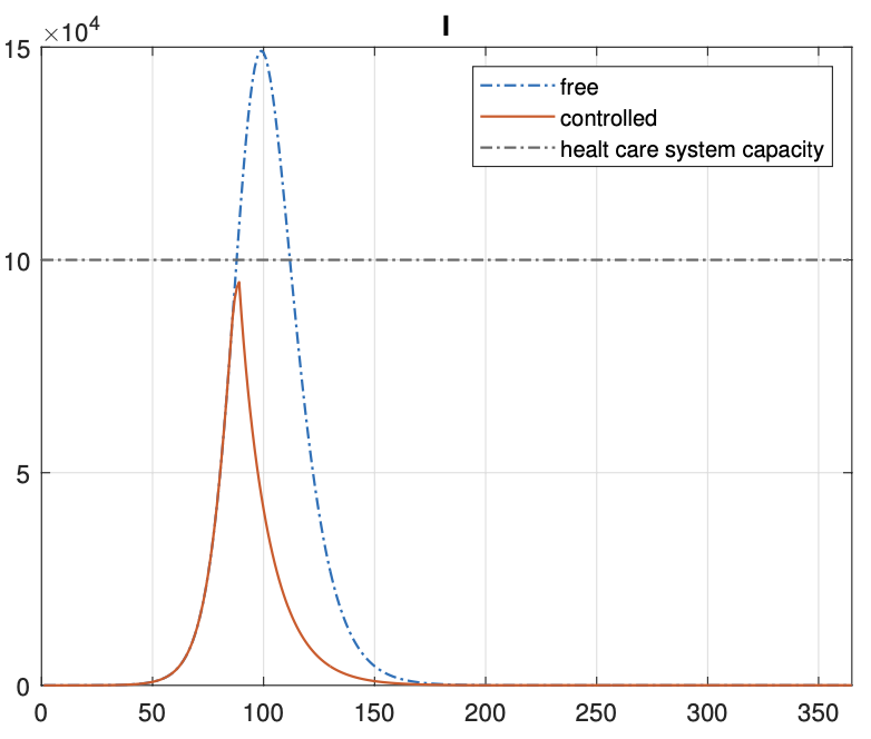
Optimal Control of Covid-19 Pandemic
Short Summary
GOAL: Design an optimal control strategy to minimize the number of infected and loss people due to the lockdown.
- The model is a SEIR model \(x = [S,E,I,R]\) with the addition of the lockdown control \(u(t)\) and health care capacity \(v(t)\)
$$ \begin{align*}
\frac{dS}{dt} &= n - (1 - u) \beta \frac{S I}{N} - mS \\
\frac{dE}{dt} &= (1 - u) \beta \frac{S I}{N} - (\alpha + m)E \\
\frac{dI}{dt} &= \alpha E - (\epsilon + \gamma + m + v)I \\
\frac{dR}{dt} &= (\gamma + v)I - mR
\end{align*}
$$
- The cost function used is though to reduce as much as possible the number of infected and exposed, while also avoiding too strict lockdowns and overloading the health care system
$$ J = \int_{t_0}^{t_f} \left\{ E(t) + I(t) + \frac{A_1}{2} u^2(t) + \frac{A_2}{2} v^2(t) \right\} dt
$$
- By applying the Pontryagin principle we can find the optimal control law \(u^*\) and \(v^*\), which are the solution of the Hamiltonian system, and the resulting closed loop system is
$$ \begin{align*}
S_{i+1} &= \frac{S_i + h n \frac{I_i}{1 + h(m + (1 - u^*_i)\beta \frac{I_i}{N})}}{1 + h m} \\
E_{i+1} &= \frac{E_i + h (1 - u^*_i) \beta \frac{S_{i+1} I_i}{N}}{1 + h(\alpha + m)} \\
I_{i+1} &= \frac{I_i + h (\alpha E_{i+1})}{1 + h(\epsilon + \gamma + m + v^*_i)} \\
R_{i+1} &= \frac{R_i + h ((\gamma + v^*_i) I_{i+1})}{1 + hm} \\
\lambda_{n-i-1}^{1} &= \frac{\lambda_{n-i}^{1} + h ((1 - u^*_i) \lambda_{n-i}^{2} \beta \frac{I_{i+1}}{N})}{1 + h d + h(1 - u^*_i) \beta \frac{I_{i+1}}{N}} \\
\lambda_{n-i-1}^{2} &= \frac{\lambda_{n-i}^{2} + h(1 + \alpha \lambda_{n-i}^{3})}{1 + h(\alpha + m)} \\
\lambda_{n-i-1}^{3} &= \frac{\lambda_{n-i}^{3} + h(1 + \lambda_{n-i}^{1} (1 - u^*_i) \beta \frac{S_{i+1}}{N} + (\gamma + v^*_i) \lambda_{n-i}^{4})}{1 + h(\epsilon + \gamma + d + v^*_i)} \\
\lambda_{n-i-1}^{4} &= \frac{\lambda_{n-i}^{4} + h m}{1 + h m} \\
M_{i+1} &= (\lambda_{n-i-1}^{1} - \lambda_{n-i}^{1}) \frac{\beta I_{i+1} S_{i+1}}{N A_1} \\
r_{i+1} &= (\lambda_{n-i-1}^{3} - \lambda_{n-i}^{4}) \frac{I_{i+1}}{A_2} \\
u^*_{i+1} &= \min(1, \max(0, M_{i+1})) \\
v^*_{i+1} &= \min(1, \max(0, r_{i+1}))
\end{align*}
$$
Last Update: July, 2020
Control of a discrete time Mass-Spring-Damper system with input delay
The mass-spring-damper system is a classic example in control theory, and it is often used to demonstrate the behavior of different control strategies. In this project, I explored the control of a discrete-time mass-spring-damper system with input delay
Short Summary
Goal: The goal was to design a controller that could stabilize the system and ensure that it behaves as desired, despite the delay in the input signal.
- Model: The system is modeled as a discrete-time mass-spring-damper system with the input delayed by \(d\) time steps.
$$ \begin{equation}
\begin{bmatrix}
\dot{x}_1 \\
\dot{x}_2
\end{bmatrix} =
\begin{bmatrix}
0 & 1 \\
-\frac{k}{m} & -\frac{b}{m}
\end{bmatrix}
\begin{bmatrix}
x_1 \\
x_2
\end{bmatrix} +
\begin{bmatrix}
0 \\
\frac{1}{m}
\end{bmatrix}
F(t-d)
\end{equation}
$$
- The control strategy involved designing a state feedback controller to stabilize the system and ensure that it behaves as desired, regardless of the input delay. here I have explored Predictor-Preview Controllers, in particular focusing on Switchd-Low-Gain Feedback
Last Update: December, 2020
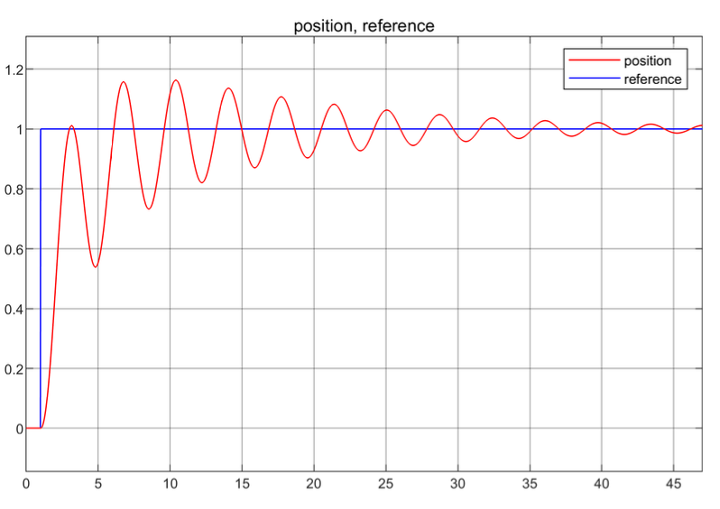
Robot learning techniques and MPC for set point regulation of robots with nonlinear flexibility on the joints
Set-point regulation for flexible joints robot is a classic control problem in underactuated robotics. In fact, the noncollocation of the torque inputs and the elastic coupling between the motor and the link makes this kind of system very challenging to control, with respect to the rigid ones.
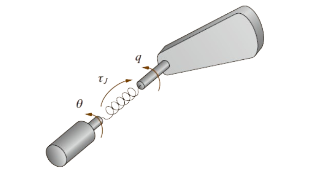
The Spong model of a flexible link
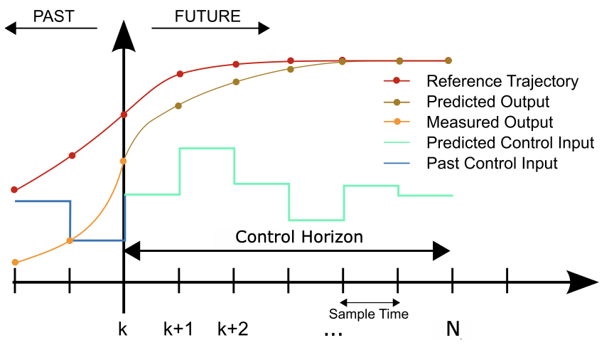
MPC strategy
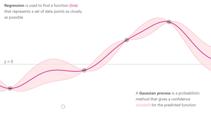
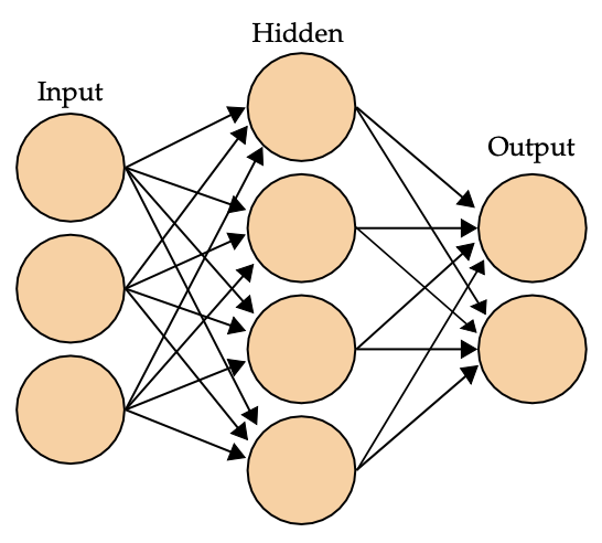
Learning techniques tested, conceptual difference between GPR and NN
Short Summary
Goal: The purpose of this project is to study how a data-driven control technique can be applied when the system model is not precisely known, exploiting a robot learning method developed at DIAG, analyzing its applicability and performance in this context. In particular, the latter is used to estimate the nonlinear elastic term of the robot model and combined with a Model Predictive Control (MPC) strategy to regulate the robot’s joints to a desired set-point.
- The system is modeled as a flexible joint robot with a nonlinear elasticity term, so it can be divided into two subsystems coupled by the nonlinear elastic term.
$$ \begin{align*}
M(q) \ddot{q} + c(q, \dot{q}) + g(q) + \psi(q - \theta) + D \dot{q} &= 0 \\
B \ddot{\theta} - \psi(q - \theta) + D \dot{\theta} &= \tau
\end{align*}
$$
- The control strategy involves using a Model Predictive Control (MPC) approach with tail cost formulation. In particular, the tail is chosen as the terminal cost of the constrained linear-quadratic regulator (LQR) computed on the linearized system.
$$ V(x, u) = \sum_{i=0}^{N-1} \ell(x(i), u(i)) + \sum_{k=N-1-K}^{N-1} V_f(x(k), u(k))
$$
Getting the control input by minimizing the cost function
$$ \begin{align*}
\text{minimize } & V(x, u) \\
\text{subject to } & x(k+1) = f(x(k), u(k)) \\
& h(x, u) \leq 0
\end{align*}
$$
- The learning technique used to estimate the nonlinear elasticity term of the system is the Gaussian Process Regression (GPR), which turned out to give better performance than standard machine learning techniques, due to its ability to imporove without overfitting while increasing the number of data points sampled from a fixed size workspace, such as for the case of a manipulator.
Once the kernel function \(k(\cdot, \cdot)\) is chosen, the mean and the variance of the prediction are given by
$$ f(x^*) = k^{T}(K)^{-1}y
$$
$$ V(x^*) = k(x^*, x^*) - k^{T}(K)^{-1}k
$$
Last Update: June, 2021
Other Projects
Here are minor projects, mostly theorethical, that I have been working on during my studies.
Cooperative attitude synchronization in satellite swarms: a consensus approach

Problem: Autonomous synchronization of attitudes in a swarm of spacecraft
Solution: Two types of control laws, in terms of applied control torques, that globally drive the swarm towards attitude synchronization
- Solution 1: requires tree-like or all-to-all inter-satellite communication (most efficient)
- Solution 2: works with nearly arbitrary communication (more robust)
Last Update: June, 2021
A New Method for the Nonlinear Transformation of Means and Covariances in Filters and Estimators
The goal of this project was to make a report, finding the novelty introduced in the paper. This paper presents a novel method for generalizing the Kalman filter to handle nonlinear systems effectively. Unlike the traditional Extended Kalman Filter (EKF) that relies on linearization, this approach uses a set of deterministically selected samples (sigma points) to parameterize the mean and covariance of a distribution, thus allowing a more accurate and straightforward implementation without the need for Jacobians. The method provides a significant improvement over EKF, particularly in systems with pronounced non-linear characteristics where EKF may introduce substantial biases or errors. The new approach is demonstrated through simulations showing enhanced prediction accuracy and robustness in tracking and estimation tasks.
Short Summary
Goal: Develop a generalized Kalman filter method for nonlinear systems without relying on linearization.
Results: Uses sigma points to capture the true mean and covariance of the state distribution, avoiding the need for linear approximations. Demonstrated superior performance to EKF, especially in handling non-linearities. Provides a more straightforward implementation approach, as it does not require the computation of Jacobians.
Last Update: June, 2020
DC-motor and 4-tanks system control with \(H_\infty\) and \(\mu\)-synthesis techniques
This is a veeery long series of homework aimed at specializing in the control of MIMO systems with the \(H_\infty\) and \(\mu\)-synthesis techniques. The first part of the project is about the control of a DC-motor, while the second part is about the control of a 4-tanks system.
Last Update: June, 2021
Implementation of CNN, LSTM and free design of a neural network architecture
A series of homeworks aimed at specializing in the implementation of neural networks, in particular Convolutional Neural Networks (CNN) and Long Short-Term Memory (LSTM) networks. The last part of the project is about the free design of a neural network architecture.
Last Update: January, 2020